Historical Perspective

    The purpose of this post is to provide a synopsis of the evolution of program aspects as they relate to maintainable programs.  This is also intended as a prelude for how design object oriented programs for maintainability.

    As always the information here is based on my own experience.

    In the beginning programs were written in machine code or assembly code. This type of code is characterized by:
1. minimal separation of code and data.
2. any data or code element is accessible from anywhere in the code.
It worked well for small applications but as the code grew in size and complexity it required a lot of skill and discipline to create anything close to maintainable code.

    By the time I learned programming, FORTRAN and COBOL were widely used. Both of these are high level languages. Both of them had subroutines which organized code such that access to code inside them was not possible.  Both had data structures which when combined with, subroutines provided limited data access.  The main significant effect was to allow a separation between application data and control data (loop indexes and variables used to control logic flow).

    COBOL introduced the concept of records. This provided a way to organize dissimilar data primitives in a single data structure. To me this is significant because it led to what was a major mile stone of maintainable software.  Most often these records were stored in files and these files were used by different programs this created a huge amount of maintenance work. The solution to this problem was the concept of a data base. A block of data was added to the front of the normal record data which mapped record field names to offsets in the record. Basically this provided a symbolic name for fields in a record.

    After these simple beginnings, the number and nature of programming languages expanded rapidly.  Some of the most successful of these language types are: Function, Rule and Object based.
These and many others were created to meat specific needs and are often problem domain specific.
All of them are useful but when taken to the extreme or misapplied can result in code which is at best difficult if not impossible to maintain.

    Function based languages (such as LISP) became popular at least in academic circles. The main characteristic of such languages is that all code is represented as functions. In a pure functional world this means that a functions contain no state information which in turn means that when called with the same arguments the same result is returned. When studying such code it is easy to predict what the code will do. However, because of how logic control must be represented, in many cases it makes logic changes difficult to do correctly. The other situation it breaks down is when reading files because making repeated read calls will nearly always produce different results.

    Rule based languages (such as PROLOG) came into wide use in Artificial Intelligence applications. Programs written in these languages consist of a set of 'rules' of the very general form
"if <condition> then <action>" . In most cases the if and then are only implied. Probably the most widely used applications of this type are "make scripts".  The order in which the <actions> are executed in is depends on the initial data supplied and the results/side effects of preceding actions.
Applications involving few (perhaps less than 30) rules are very easy to maintain. As the number of rules increases, the more difficult it becomes to predict what the exact effect of a given change will be.

    Object based languages (such as JAVA) are currently popular. In all cases, the main objective is to encapsulate code and data structures. Some of then separate code and data, others make no such distinction. An other main characteristic of these languages is the that objects either can or must be created at run time.  Both of these characteristics can be a great help in creating maintainable software. Like all programming ideas/paradigms I have worked with or read about, can when taken too far can result in programs which are very difficult to maintain.

State Machines

Commentary and Observations on State Machines

State machines are one way of implementing an iterated and complex control flow that is more maintainable than equivalent functionality using just if statements.  For  information on state machines see the wiki page.

This is just a commentary on my experience with state machines.

First of all, in many situations, using state machines is a good implementation choice.

The classic state machine can be described as a set of actions whose order of execution is controlled by an input value, a current state, and a transition table.  This type is often used in programs to implement a text parser.

For simplicity in this description, both the current state and the input value are treated as integers.  The basic sequence is as follows:

1. Set the current state to 0

2. Start the loop

3. Set the input value (read from a file or get the next character in a string variable)

4. Set the current state to the value found in the transition table by using the input value, and current state value

5. Select/jump to the block of code associated with the current state.  This code will take appropriate action and then jump to the end of the loop

6. Return to the top of the loop (Step 3 above) if some loop termination condition is not met

The main variants of this algorithm are that:

• the input value may be something other than a character
• the termination condition may not be “end of string” or “end of file”

For example, in my Adventure 3 posting, the original state machine implementation had the following changes:

• The input value was the “current state” of the device
• The next state was determined by the “input value” and the desired “state” of the device
• The termination condition was that the input value (the “current state”) matched the desired “state”

In the above type of state machine, maintenance problems become evident if the number of states is large or if the numeric range of the input value is large.  

If the number of states is large, it is difficult to understand what the code is doing because the execution sequence is encoded in the transition table and the actions are represented as numbers.  The difficulty arises because of the need to remember exactly what actions all those numbers represent, and, therefore, changes to the transition table or the code for a given state can easily have unintended side effects. 

If the numeric range of the input value is large, then there can easily be a problem with the coding of the transition table itself.  There is likely to be a lot of duplication e.g. all alphabetic characters have exactly the same transition except in certain states.  In some applications, it may not be physically possible for every value in the input to occur (e.g. even though the input value is a byte, the number of possible values is small, and the values are not numerically consecutive (See Adventure 3.) . This condition results in large logical gaps in the transition table and a very memory-consuming transition table. To overcome this problem, I have sometimes used an input translator function that accepts the input value and produces a translated value (e.g. all alphabetic characters are assigned the same translated value).  This translated value is what the state machine uses.

In my Adventure 2 posting, I describe a new (for me) type of state machine that eliminates or reduces the problems inherent in a classic state machine.  This “new” machine also makes a state machine implementation a viable option in a wide variety of situations. Its design came about (in part) when I realized that a state machine representation could be used to flatten a calling stack (when one routine calls another ). This design is summarized here.

  

In this type of state machine, there is no input value.  The execution sequence is controlled by a “current state” and a “next state.”

1. Set the next state to 0

2. Start the loop

3. Set the “current state” to “next state”

4. Select/jump to the block of code associated with the current state. This code will take appropriate action and then may set the next state before jumping to the end of the loop.

The action of at least one of the states is to exit the loop.

Note: If the next state is not changed, then state action will be repeated.  This can happen when a state machine is used to implement a polling loop.

In practice, the appropriate action was often implemented by a function call and its return value was used to determine a value for “next state”.

The benefits of having the state code decide what the next state would be are as follows:

• Transition sequences are relatively easy to follow, and, therefore, code changes are less likely to have unintended consequences
• There is no transition table to maintain
• There is no need to specially handle sparse values in an input value (even if one were used).

Miscellaneous Observations

·        I have used a state machine design to analyze a problem, and several times this analysis showed that the problem could be solved by just a few if statements.

·        When could a state machine pattern be used?

o   If the code is processing some kind of input stream and I find that I am writing a series of “if statements” to decide what to do

o   If processing decisions must be made based on the values of one or two variables and the action to be taken is determined by the values of the variable(s)

·        When should a state machine pattern NOT be used?

o   If there is no “input stream” then the problem might be too simple to justify the use of a state machine

o   If there are more than two controlling variables used to decide what action to take and the problem cannot be factored into multiple simpler problems

o   If the controlling variable(s) can be changed by external actions (e.g. other processes or threads)

Maintaining Software, Adventure 3

   This adventure came about because a project which was supposed to be a relatively straight forward maintenance problem wasn't.  The company I worked for had purchased the software source, documentation etc. .  We (the engineering staff) were supposed to just tweak it a bit, add support for some new devices then release it.

   The software was designed  to automate much of the work in a data center by creating and automatically maintaining subsets of the equipment as 'farms' i.e. collections of computers, disc drives, network devices etc in a virtual network.  A customer used a Visio like interface to describe the desired configuration and the software system used an XML version of that description to create what was described.  After a 'farm' was created, a customer could edit the description and have the changes made on the fly to the still running 'farm'.  A major aspect of the system was that it could automatically recover from if any single point of failure. This included a failure of any device (computer, network device etc) or cable including any of the infrastructure parts failed, full functionality would be automatically restored as much as available spare parts allowed.

   The difficulty in doing this correctly was seriously under estimated and every other such project of this type I have heard about since then has also underestimated the difficulty.  In this case every major subsystem was rewritten at least once or was subject to one or more major rework efforts.

   My part was 'farm management' which meant being responsible for coordinating the work done by all of the subsystems as they related to 'farms'.  A separate subsystem was responsible for infrastructure components. The simplest description of what 'farm management' did is to say that the front end (human interface part) constructed an XML file and then issued command(s) to my part for implementation.  The other main input to 'farm management' came from the monitoring subsystem.  When ever it detected a failure in a component or cable it issued a command to 'farm management' saying that component 'xxx' had failed. 'farm management' then took appropriate action.

   This functionality was implemented for the most part by a set of state-machines each of which was implemented in an object by case statements.  There were a set of status values defined and the state-machines purpose was to take components from one status to another.  A typical 'command' from the user would require a specific sequence of these transitions.  e.g. from New to Allocated to ... Active. When a device was no longer needed, the steps were basically run in reverse order for that device.  A failed device was left in an Isolated status e.g. powered on but not connected to the network.

   As delivered, the code worked as expected unless a component failed while it was participating in a 'farm' configuration change which included that component.  A very simplified description of the problem is that the incorrect behavior occurred because the code was designed to take all relevant devices in a 'farm' from one well known status to another well known status.  It could not handle the situation where some component(s) needed to move through the state-machine system in a direction opposite to all the other components at the same time. There were other corner case scenarios involving a change or a failure in the infrastructure which could also cause these state-machines to become confused.

  The complete solution required changes in some data structures and a complete replacement of the state-machine design.

• The first step of the solution came from recognizing that the predefined 'farm state' values did not cover all the possible situations and not all component 'states' were explicitly represented by the 'farm state' values.
• The next step was to recognize that each component type had a small number of associated 'state' values each of which could be represented by a Boolean value such as:  working yes/no, power on/off, configured yes/no.  The investigation which led to this understanding was forced by the Data Base team refusing to increase the size of a component description record. I just changed the type from an enumerated type (byte sized integer) to a Boolean 8 bit vector.
• The above change to allowed the current 'state' of a component to be accurately represented by the set of bits in its 'state variable'.  This in turn allowed the work of the software to be defined as doing what ever is required to change a components current status to a final status and to make the required changes to individual 'state (bit) variables' in the required order.

  The above changes allowed the current status of a component to be accurately determined but did nothing to solve the problem of devices in a given 'farm' needing to be transitioned through different sequences simultaneously.

  The solution to this problem was to use simplified Artificial Intelligence (AI) techniques for control and synchronization and by using what might be termed massive multithreading techniques.  All of the code in this project was written in Java so the problem was not as difficult as it might have been but was not trivial either.

The details of these changes will be given in a later posting.

Helping Maintainers

There are two broad categories of documentation which exist and are or can be maintained outside the code. 

         These can broadly be defined as User Help/Specifications and Design/Architectural Descriptions. This blog posting is about Design/Architectural Descriptions.  A previous posting covered User Help/Specifications.

         This type of documentation is intended for use by maintainers and to a lesser extent by project stake holders.  From a maintainers perspective, this type of documentation is useful only if it leads to a quicker (than just reading the code) understanding of what the major software and hardware elements are and how they relate to one another.

         The characteristics of  software architecture documents are:

1. Highest level of abstraction
2. Focuses on the components needed to meet requirements
3. Describes the framework/environment for design elements
4. No implementation information

         The characteristics of software design documents are:

1. Lowest level of abstraction
2. Focuses on the functionality needed to meet requirements
3. May only hint about implementation

As appropriate it should have diagrams and/or descriptions of the major modules and how they relate to each other both structurally and at run time ( data and/or control flow relationships ).
       
          For large and structurally complex applications which have been written in an object oriented language, there are tools which will generate UML class diagrams of the modules similar to the following.


For maintenance purposes on large/complex systems I have found these diagrams to be useful only as a starting point for checking references to a method as part of a proposed defect fix.  I say starting point because it mainly serves as a way to estimate potential effort.  More times than I care to think about, I have written a Perl script to scan all files in a project for a given symbol or set of symbols.  The Linux grep command can be used to do much the same thing.  Both of these scans can also check external documentation files. The virtue of the Perl script is that it can be easily modified to make the desired change to the code and comments.

I am not saying that auto generated UML diagrams are useless, only that they should not be the only external documentation for a project intended for maintainers.  Consider who the maintainers might be.  It may be that not all maintainers under stand UML diagrams.  It is possible that some maintainers will have expert specific domain knowledge but not much software expertise.

Consider management type people .....

• 
  

Maintainable Software, Adventure 2

This adventure in maintainable software is included because some very stringent requirements and a couple of significant requirements which came in late in the project lead to a highly maintainable architecture/design.  This was a firmware project for what was called a BootROM in an embedded system.  One aspect of this type of application is that unless you count the system code which is loaded, there is no application data but some configuration data.  

The restrictions and requirements were roughly as follows:

o   The system buss was VME which is/was the standard for large embedded systems

o   The RAM available for firmware use was very limited.  There was enough for roughly 3 stack frames as generated by the C compiler which limited the calling depth

o   There was no practical limit on ROM address space

o   There was a good amount of flash memory for configuration data

o   It required using three languages (assembler, C and Fourth)

o   It must support simultaneously an arbitrary number (0 to n) of Human Interface devices (keyboards, displays, and RS-232 ports.  Late in the project was added remote console (LAN) interfaces.  All of these interfaces were to remain active even while the OS/user system was being loaded

o   It must be capable of finding an arbitrary number of bootable systems on each of an arbitrary number of bootable devices (disks and remote (LAN) servers)

o   It must be capable of accepting input from keyboards configured for any of dozens of human languages and displaying messages in those languages.

o   It must be capable of running diagnostics for any user supplied device which appeared on the VME bus.

o   Late in the project a requirement was given to support what was known as hard real time.  What this mostly meant was that the system as a whole must be capable of going from power on to user code running under Linux in under 30 seconds. What this required of the firmware was to ignore HI devices and to disable all diagnostic code except for devices directly involved in the boot process

o   Oh! And if possible allow users to modify the code

The requirement for Forth came about because at the time there was a push for a way to allow device interfaces to contain their own driver code.  This was to be the way in which interface testing and boot support was to be supplied so that firmware did not have to be constantly updated for new or changed devices.  A group of manufactures and suppliers including, Hewlett-Packard and Apple had come to an agreement that Forth would be the language used to implement this capability.  Also at this time a IEEE standard for Forth was accepted. 

The problem of supporting keyboards for any language was solved by using a pure menu based human interface system where menu items were selected by keying a number.  This worked because all keyboards have the same key position for the numbers (excluding number pads).

A breakthrough solution for the stack depth problem came when I realized that if code was broken up into small functions that a state-machine could be used to represent calling sequences and the stack depth could then be limited to a single level.  A refinement of this design was to limit the number of function arguments to three because the C compiler always put the first three arguments into registers rather than on the calling stack thus further reducing the stack frame size.  The state machine description could be stored in ROM. 

The rough process used to create such a representation was to translate each subroutine into a state machine representation by refactoring each straight line code segment (code between routine calls) into a function and replacing each subroutine/function call with the state machine representation of that routine.  This was rather laborious but fortunately most routines were small and straight line.

The following is a simple abstract example of this flattening and state machine representation:

‘Normal version’ for simplicity it is assumed that only sub2 calls another routine.

subroutine A(arg1)

    code seg1

    v1 = func1(arg1)

    if (v1=1) call sub2(arg1) else call sub3(v1)

    code seg2

    call sub4(v2)

end sub A

subroutine sub2(argx)

     code seg3

     call sub5

end sub2

‘State machine version’

Code segments 1, 2, 3 etc. are refactored as functions.   Most often the return value is a 0 or 1 indicating success or failure.

Rv is the return value while Arg1 and V1 are a ‘global’ variables

StateA1

     Rv=seg1();  stateA2

StateA2

     Rv=func1(Arg1) ;  1,stateS2.0; 0,stateA3

StateA3

     Rv=Sub3(V1); 1,stateA4

StateA4

     Rv=seg2(); 1,stateA4

StateA5

     Rv=Sub5(); 0

The 0 or here indicates completion for the machine

State S2.0 // this implements sub2

     Rv=seg3(); state S2.1

State S2.1

     Rv=Sub4(); stateA4 // this is the return from sub2

Another innovation was in the state-machine representation and its ‘interpreter’.  In conventional state-machines, the ‘interpreter’ operates by calling a routine which returns an value (often a character from an input source) this value along with the number of the current state is used to index into a two dimensional array to fetch the number of the next current state, this number is also used to select and call a routine which is the action associated with the state.  This process is repeated until some final state is reached. 

The main problem with this design is that as the number of states increases the number of empty or can’t get there values in the state table increases along with the difficulty in understanding what the machine is doing.  Documentation can help but must be changed every time the state machine is changed.  The solution I came up with was to represent the state-machine as a table of constants in assembler language and use addresses instead of index numbers.  Each state has a name and contains the address of the function to call, its arguments and a list of value-next state pairs.  The following examples and explanations may be a bit tedious for some people but they form the basis for my solution to the multiple HI devices problem as well as solving the stack size problem.

In this example the dc stands for Define Constant and the -* causes a self-relative address to be produced, this will be explained later

stateX1     dc ‘op1 ‘ //arg1

            dc 1      //arg2

dc 0      //arg3  not used

            dc myfunc-*

            dc value1,stateX1-*  // repeat stateX1

            dc value2,stateX2-*

            dc 0,0 // end of list

The calling a routine for an input value was eliminated and the ‘interpreter’ ran by using the current state address to select the function to call but then used the return value from that call to select the next state from a list tailored to that functions return values.  This minimizes the amount of space to represent the state machine and makes it somewhat easier to follow a sequence of transitions.

The requirement to support simultaneous use of multiple HI devices even while the OS/system is being loaded provided a significant challenge because there was not enough available RAM as well as other issues which prevented using an interrupt based mechanism like the Operating Systems do.  Firmware had to use a polling mechanism which meant that the user ‘lost control’ while the OS was being loaded as well as at other times.  The requirement to support a LAN based console was over the top because driver code in general had never been implemented or even designed to be used for two different purposes at the same time.

The multiple simultaneous HI device ‘problem’ was solved primarily by changing the state machine to support a cooperative multi-threading mechanism and then creating a thread for each input device and a separate thread for the selected boot device.  Each input device thread was a two state state-machine which called the driver requesting a character.  If one was not found, the next state is the same as the current state and when one was read, the next state called a function which invoked the menu system then transitioned to the first state.

This worked because the state-machine interpreter was modified to work with a list of state machine records.  I do not remember the details of how it was implemented but even now I can think of at least three ways it could have been done.  The essence is that the interpreter would pop the next state address off a list and execute the state selected.  After executing the state, new next state address was put on the end of the list and the cycle would be repeated. The effect of this was to switch threads on state boundaries and therefore after each function call.  The LAN driver was converted to state-machine format and refactored to have both boot protocol and console protocol components thus allowing the console and boot operations to work simultaneously.

At the time of this design, there was great interest in using ‘building blocks’ as a way to construct easy to build and maintain systems.  No one had as yet actually tried or even come up with a concrete proposal.  Because we anticipated a huge maintenance work load after the first system release I decided to try to come up with something for this project.

                  The resulting architecture initially consisted of a ‘core’ block an English language block, a set of               driver blocks and an end block. 

                                                

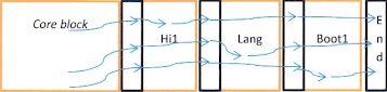
The Core block contained normal BootROM stuff, including basic initialization, the Forth Interpreter and various general utility routines which could be used by all blocks.  The End block was nothing more than a set of null pointers to terminate all the lists.  There were in fact several more linked lists than are shown in the above diagram.  All of these links were self-relative pointers and were paired with a bit pattern which indicated if there was anything of interest at that address for example text for English or code for a human input device.  Each block relied on the assumption that there would be a set of pointers immediately following its own code.   Each block was compiler/assembled independent of one another. The ‘ROM’ was constructed by extracting the code from compiled files and literally concatenating them between the Core block and the End block.  This architecture required code and addresses such as the ones in the state-machine tables and the lists running thru the blocks to be self-relocating.  The compiler generated self-relocating code.  The self-relocating requirement for addresses was met by making them self-relative (add the value at an address to its address to produce the required needed address. The null pointer was detected by checking for zero before the addition step.

The ‘multiple human languages’ requirement was met in part by the HI input device mechanism described above and in part by using a pure menu system and in part by the following mechanism.

All of the text for all human visible messages was placed in a table and referred to by a number.  This text consisted of phrases and single words which could be combined as needed. Messages as stored in the table could be either text or a string of message numbers.  When a message needed to be displayed, a call would be made to a print routine in the Core block and giving it the message number.  This routine would find the language table for the currently configured language,  construct the text version of the message then find all the console output devices and have them display the message.

These messages and message fragments were developed by Human Factors specialists.  I developed a simple emulator (in Perl) which would behave like the ROM in terms of how the menu system worked and how it would react to error conditions.  These specialists then had complete control over the message text.  This allowed parallel development of code and user manuals.  When the time came to deliver the ROM,  I used a Perl script to extract the messages and generate the English language block.  The same or very similar process was used to generate the French language block.

The last requirement (“Oh! And if possible allow users to modify the code”) was put in place by creating a developer’s kit which consisted of a lot of documentation, the ready to concatenate files used in the ‘standard’ ROM and the scripts used to create them.

Historical notes:

o   Shortly after the first release of this ROM, Apple came out with the first device which was to support the Forth language concept.  Instead of Forth, their ROM contained machine code.  Their comment was ‘we never intended to support Forth’.  That killed the initiative.

o   The system this ROM was part of was designed to work in hostile/demanding environments primarily for data collection/management purposes.  As I recall, it was used in monitoring tracks for the Japanese bullet trains, doing something in the latest French tanks, monitoring and controlling sewage treatment plants, collecting and displaying data for an Air Traffic control system and collecting and displaying data in the US Navy Aegis weapon systems.

o   I did train engineers for one company to allow them to build their own ROMs.

o   About a year after releasing this project, the division was disbanded but maintenance was transferred to another division.  About five years after this I talked with an engineer who had been assigned to maintaining the ROM and he said that he had been maintaining it by himself for a few years and had released new modules and had easily made several releases per year by himself.

Summary of things done and learned:

o   Used Assembler, Forth and C in the same application.

o   Designed and implemented what may be the only true ‘building block’ system.

o   Learned that separating control logic from computational logic helps maintainability.

o   State-machines are a viable way to keep control and computational logic separate and make the control logic very visible.

o   Simple emulators can be used to see what an application will look and behave like before and while the application is being built.  They can be cost effective because the allow scenario testing before the code becomes too rigid.

o   Learned a lot about multi-threaded systems work in a very controlled environment

o   The building block architecture proved to be a very good way to improve maintainability

Maintainable Software, Adventure 1

This is the first in a series of at least three projects which most strongly influenced my views of software maintenance.  I have titled them Adventures in Software Maintenance.

  Denison Mines Open pit mining, washing plant etc.

The adventure here is that until about half way through the project (several months) I did not have anything close to a full set of requirements.  The requirements were given one small part at a time with coding and testing done before the next requirement was given.

While working for Computer Sciences Canada in the late 1970s, I was given the assignment to be a consultant and contract programmer for a company then known as Denison Mines. At the first meeting the man who was to be my manager at Denison Mines told me that he knew very little about computers but was confident that they could solve his problems.

The first assignment was in essence to create a ‘graph’ of a curve with two inflection points and to do this for several hundred data sets which had only two data points.  I of course having studied such things in college told him it could not be done.  He said we were going to do it anyway because each pair of data points cost several thousand dollars to produce.  We did it in a few months by using a few complete data sets, some other empirical data and the help of a Japanese mining engineer they brought in from japan.

Over the course of several months the manager kept adding other things which needed to be done and added to the growing program, such as adding a mathematical model for a coal washing plant, a mathematical model of the geology of a few mountains and algorithms for designing open pit mines.

After a few visits it became obvious that this incremental requirement discovery process was going to continue and it was going to be impractical to keep re-writing the program. The solution was to design a simple command reader which would read a command (from a file) then make the appropriate subroutine calls.  There was too much data to pass into the subroutines so the application data was read into global structures and the routines manipulated the data in those structures.

Looking back on this project from a maintainability perspective, the most volatile program area was in the command interpreter where new commands were added.  This worked because the highest level flow control was shifted outside of the program and into the command file (there were no conditional or looping statements in this language). The second most volatile area was the data structures.  Changes were made to array sizes or to add new arrays and entries in the common blocks or new common blocks.  In more modern languages the changes to the common blocks would be to add fields in a record or data only module. The least volatile area was the computational subroutines or algorithmic code as I now call it.  The changes most often were to add routines to execute new commands.

One side effect of the command stream architecture was that depth of subroutine/function calls was very shallow, seldom going more than a couple of levels.  This in turn made it easier to test new code.

The result of this design/architecture was that very little maintenance work was done or needed even after several years.  A historical foot note is that this program was used to design two major open pit mines and the associated coal washing plants. For more information about this see http://en.wikipedia.org/wiki/Tumbler_Ridge,_British_Columbia and this http://www.windsorstar.com/cms/binary/6531189.jpg?size=640x420 and this http://www.ridgesentinel.com/wp-content/uploads/2012/04/WEB-04-April-27-Quintette-and-PH.jpg  

Summary of things done and learned

o   Language: FORTRAN using block common (data only single instance records)

o   The value of validating (e.g. range checking) application data as it is read

§  This allowed the algorithmic code to be as simple as possible by focusing exclusively on processing the data

o   The value of using a user input stream for top level control

§  This reduced the effort required to test new code by allowing execution of new subroutines to be isolated from existing code

§  This enabled changes caused by the introduction of new functionality to be very localized within the program. Most changes were limited to the new subroutines and a simple addition to the command interpreter.

o   The value of separating control and computational (algorithmic) code

§  This was mostly a side effect of the command stream architecture

o   The value of storing application data in global space

§  Because most of the data was stored in arrays, this allowed a kind of ‘pipeline’ processing and all but eliminated the passing data up and down the calling stack.  The trade-off is that more than ordinary attention must be paid to how data is organized and that subroutines only work on very specific data elements.

The application data naturally occurred in one and two dimensional arrays. The raw geological data was presented as a set of vectors for each drill hole, a location followed by a vector of numbers representing what was found at varying depths. This data could then be filtered and processed to produce ‘topology’ maps or simplified arrays representing seams of coal which had specific qualities which could be written to a file for later processing and/or producing various reports.  In all cases original input data was never altered.